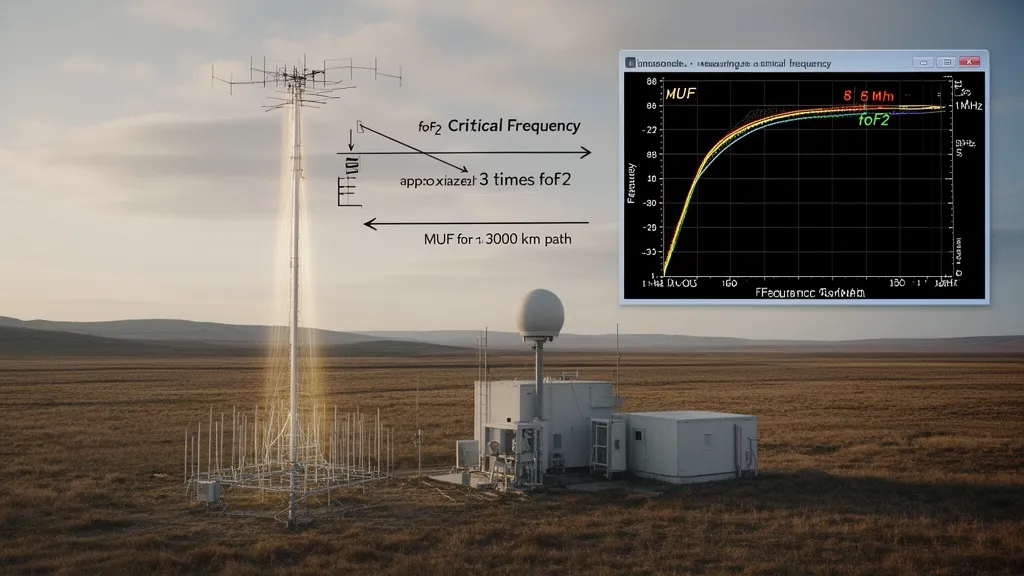
Operator’s Verdict: foF2 is the single number that determines whether a given band is open or closed over any path. You do not need an ionosonde at your QTH to use it — the GIRO network, DXRadar, and tools like IRI-2016 provide foF2 estimates in real time. If foF2 at your path midpoint is 10 MHz, 10m is closed; if it is 14 MHz, 10m is wide open. That is the complete story.
What foF2 Is and How It Is Defined
foF2 — the critical frequency of the F2 layer — is the highest frequency at which a radio signal transmitted vertically upward is reflected back to Earth by the F2 ionospheric layer. At frequencies above foF2, the signal passes through the F2 layer entirely and is lost to space. At frequencies at or below foF2, the signal is reflected back to Earth by the ionospheric plasma.
The physical definition is rooted in the dispersion relation for electromagnetic waves in a magnetized plasma. The ordinary wave (O-mode) is reflected when the wave frequency f equals the plasma frequency fp:
fp = (1/2π) × √(Ne × e² / ε₀ × me)
where Ne is electron density (electrons/m³), e is electron charge, ε₀ is permittivity of free space, and me is electron mass. At the F2 peak electron density (NmF2), this plasma frequency is foF2:
foF2 (MHz) ≈ 0.009 × √(NmF2 (electrons/m³))
At typical daytime NmF2 values of 10¹² electrons/m³, foF2 is approximately 9 MHz. At solar maximum daytime midlatitude values, NmF2 can reach 2–3 × 10¹² electrons/m³, putting foF2 at 12–16 MHz. At night, NmF2 drops to approximately 10¹¹ electrons/m³, giving foF2 of 2–4 MHz.
The practical consequence for radio operators is immediate: foF2 is the hard upper limit for vertical propagation, and it scales with solar activity and time of day in a predictable manner. The entire architecture of HF band planning — which bands are open, when, and on what paths — derives from foF2 at the ionospheric midpoint of your path.
How Ionosondes Measure foF2
The ionosonde is the instrument that actually measures foF2. It is essentially an HF radar: it transmits a swept-frequency pulse vertically from 0.5 MHz up to 20–30 MHz, measures the round-trip travel time of the echo from the ionosphere at each frequency, and plots the result as a height-frequency profile called an ionogram.
The ionogram shows the virtual height of reflection (y-axis) vs. frequency (x-axis) for the O-mode and X-mode (magnetically split) traces. The frequency at which the O-mode trace terminates (the signal begins passing through the layer) is foF2. A trained ionogram analyst or automated fitting algorithm identifies this cutoff frequency and records it as the foF2 value.
NOAA’s Global Ionosphere Radio Observatory (GIRO) network operates or aggregates data from over 100 ionosondes worldwide. Stations are distributed across all continents and many oceanic islands. Data is available in near-real-time (typically 15-minute cadence) from the GIRO data center at UML (University of Massachusetts Lowell). The Digisonde — a modern digital ionosonde — automatically produces foF2 measurements with computer-interpreted ionograms and data quality flags.
The historical record of foF2 at many stations extends decades. The Juliusruh (Germany) ionosonde, for example, has a record extending back to 1957. This historical data enables statistical modeling of foF2 variation with solar cycle, season, and time of day — forming the observational basis for the ITU-R P.533 propagation prediction model and the IRI (International Reference Ionosphere) model.
Pro Tip: The Lowell GIRO data center (giro.uml.edu) provides a real-time global map of foF2 measurements from the ionosonde network. If you are planning a path and want to know the foF2 at the midpoint, find the nearest ionosonde to that geographic location and read its current foF2 directly. It takes two minutes and gives you ground-truth data rather than a model estimate.
The MUF Calculation: From foF2 to Band Prediction
The most operationally important formula in HF propagation is:
MUF = foF2 × M(3000)F2
Where M(3000)F2 is the MUF factor for a 3,000 km path — the obliquity multiplier that converts vertical-incidence foF2 to the maximum frequency that can propagate via F2 on a path of that length. M(3000)F2 typically ranges from 2.9 to 3.5 depending on the height of the F2 layer peak (hmF2) and geographic factors.
For a quick estimate, using M(3000)F2 = 3.5 is a reasonable conservative value for mid-latitude paths:
| foF2 at Path Midpoint | MUF (approx., 3,000 km path) | Bands Open for DX |
|---|---|---|
| 4 MHz | ~14 MHz | 20m barely, 40m yes |
| 6 MHz | ~21 MHz | 20m, 17m, 15m marginal |
| 8 MHz | ~28 MHz | 20m, 17m, 15m, 10m marginal |
| 10 MHz | ~35 MHz | 20m, 17m, 15m, 12m, 10m |
| 12 MHz | ~42 MHz | All bands including 10m wide open |
| 14 MHz | ~49 MHz | All HF bands, 6m F2 possible |
| 16 MHz | ~56 MHz | All HF, 6m F2 openings likely |
These are for a 3,000 km single-hop F2 path. For shorter paths, the M factor decreases (the signal hits the layer at a steeper angle), reducing MUF. For longer paths, the signal hits at a shallower angle, and MUF may be higher — but the path involves multiple hops with the MUF limited by the minimum foF2 anywhere along the route.
The 3,000 km benchmark is used because it is the standard ITU-R reference path and approximately corresponds to the most efficient single-hop F2 geometry (maximum skip distance for the layer height). Real paths vary, and propagation prediction software (VOACAP, ICEPAC, ITU-R HFBC) integrates foF2 over the path rather than using a single midpoint value.
The foF2 Diurnal Cycle
foF2 follows a predictable daily cycle driven by solar UV irradiation. Understanding this cycle is essential for timing DX operations:
Pre-dawn (~03:00–05:00 local solar time): foF2 is near its nighttime minimum: typically 3–6 MHz at mid-latitudes, 5–8 MHz at low latitudes. The F2 layer persists from the previous day’s ionization because recombination at 300+ km altitude is slow. 40m and 20m can propagate globally; 15m and above are closed.
Sunrise to solar noon (~06:00–12:00 local solar time): foF2 rises as solar UV flux increases. The rate of rise is approximately 1–2 MHz per hour at mid-latitudes during moderate solar activity. By 10:00 local solar time, foF2 may have risen from 5 to 9 MHz — opening 15m before noon.
Post-noon peak (~14:00–16:00 local solar time): foF2 reaches its daily maximum approximately 2–4 hours after local solar noon at the ionospheric reflection point. This is the classic “early afternoon peak” for HF DX on 15m and 10m. At solar maximum (SFI > 150), foF2 at mid-latitude stations can reach 10–14 MHz — putting MUF above 40 MHz and opening 12m and 10m.
Evening decline (~17:00–22:00 local solar time): foF2 falls as the solar UV input decreases. The decline is gradual — slower than the morning rise. By local midnight, foF2 has typically dropped to 4–7 MHz at mid-latitudes. 15m remains open later in the evening than 10m due to the lower frequency threshold. 20m often persists as an evening DX band well into local darkness.
Nighttime (~22:00–06:00 local solar time): foF2 stabilizes at its nighttime value. Unlike the D and E layers, the F2 layer does not disappear at night — it merely reduces. The night-time foF2 minimum is 2–4 MHz at high latitudes and 5–8 MHz at low latitudes and equatorial regions. This is why 40m and 80m carry long-distance DX overnight even at solar minimum.
Seasonal and Geographic Variation in foF2
foF2 varies significantly with season and latitude, in ways that are not always intuitive:
The Equatorial Ionization Anomaly (EIA)
One of the most important features for HF propagation is the equatorial ionization anomaly (EIA): instead of a smooth peak at the magnetic equator, the F2 layer electron density has a trough at the magnetic equator and two crests at approximately ±15° magnetic latitude. This “fountain effect” is driven by equatorial plasma drift — electric fields at the magnetic equator push plasma upward, where it diffuses along magnetic field lines to higher latitudes.
The practical consequence: stations at ±10–20° magnetic latitude (Florida, Caribbean, Mexico, Brazil; West Africa, North Africa, Southeast Asia, northern Australia) experience significantly higher foF2 — often 3–5 MHz above mid-latitude values — especially in the afternoon and around the equinox. A path midpoint in this zone gives higher MUF and longer band openings than mid-latitude ionospheric conditions would suggest.
This is why 10m opens to Caribbean and South American stations at SSN values too low to open it to European or high-latitude targets — the EIA zone provides higher foF2 along the path, supporting higher MUF even with identical solar flux.
The F2 Seasonal Anomaly
The F2 layer shows a well-known seasonal anomaly: contrary to what solar geometry would suggest, foF2 at mid-latitudes is often higher in winter than in summer in the hemisphere experiencing winter. This “winter anomaly” or “December anomaly” is caused by changes in neutral atmospheric composition — specifically, the O/N₂ ratio. In winter, the neutral atmosphere contracts and the O/N₂ ratio increases, which supports higher F2 electron density for the same UV input.
For HF operators at northern mid-latitudes: 10m and 15m openings to the southern hemisphere can be surprisingly productive in the northern winter, when the northern hemisphere F2 is actually stronger than in summer despite the lower Sun angle.
High-Latitude Effects
At geomagnetic latitudes above approximately 55–60°, foF2 behaves differently from mid-latitude predictions due to the interaction between the ionosphere and the magnetosphere. The auroral oval generates electron precipitation that can both enhance E-layer density (causing spread-F and irregular propagation) and disturb the F2 layer. Polar cap absorption during solar proton events can virtually eliminate useful F2 propagation poleward of 60–70° N for hours to days.
During geomagnetic storms, the high-latitude F2 layer is disturbed by Joule heating from auroral electrojets, which modifies the neutral wind pattern and dramatically reduces foF2 over the auroral zone and at sub-auroral latitudes. This is the mechanism underlying all storm-related HF degradation.
foF2 vs. SFI: Which Should You Monitor?
Both SFI and foF2 are valuable, but they serve different purposes:
SFI (Solar Flux Index) is a solar measurement — it describes the current ionizing output of the Sun and is the best predictor of the “background” ionospheric state. A high SFI means high UV/EUV flux, which means higher foF2 globally. SFI is updated daily from Penticton and available real-time from NOAA SWPC. It is the right metric for cycle-phase planning and multi-day trend assessment.
foF2 is an ionospheric measurement — it describes the actual current state of the ionosphere at a specific location. It already incorporates SFI effects, seasonal effects, local time, latitude, and any disturbances (storms, TIDs, etc.). foF2 from the nearest ionosonde is the right metric for today’s operating decisions. If SFI is 160 but a geomagnetic storm has depressed foF2 at the path midpoint from 12 MHz to 6 MHz, MUF is 21 MHz not 42 MHz — 10m is closed regardless of what the SFI says.
The proper workflow: use SFI as the long-range indicator (is the cycle high enough to support 10m at all?) and use foF2 (from ionosonde data or TEC maps) for real-time band selection during a session.
Using foF2 Data in Practice
A practical example: you want to determine whether 10m will be open for a DX session from your QTH in the central United States (38° N, 95° W) to South Africa (ZS6, 26° S, 28° E) at 18:00 UTC.
-
Identify the path midpoint: Approximately 10° N latitude, 30° E longitude (somewhere over northern East Africa/Ethiopia).
-
Find the nearest ionosonde: The GIRO network has stations in Malindi, Kenya (~3° S, 40° E) and Khartoum, Sudan (16° N, 32° E). Use the Khartoum data or average the two.
-
Read the current foF2: Assume the ionogram shows foF2 = 11 MHz at 18:00 UTC at that location.
-
Calculate MUF: For a path of approximately 14,000 km (not a simple single hop — use 2–3 hops, each hop approximately 4,500–7,000 km), the M factor for the dominant intermediate segments is approximately 3.3–3.5. MUF ≈ 11 × 3.3 = 36 MHz. 10m (28 MHz) is open with margin.
-
Cross-check with SFI and Kp: SFI 145 consistent with these foF2 values. Kp = 2, quiet — no storm degradation. Proceed with confidence.
-
On the air: Turn on the radio, check 10m band activity on DXCluster, listen for ZS6 signals. If they are there, the calculation was right. If not, the path may have additional limiting factors — check foF2 at other intermediate points.
This workflow takes about five minutes and is more reliable than any general rule about “SFI above 140 opens 10m.” The ionosonde data directly measures what the ionosphere is doing, not what it should theoretically be doing based on solar flux.
IRI-2016: The Standard Ionospheric Model
When real ionosonde data is not available for the path midpoint, IRI-2016 (International Reference Ionosphere) provides foF2 estimates based on empirical fits to the global ionosonde database. IRI-2016 (Bilitza et al., 2017, Advances in Space Research; updated in Bilitza et al., 2022, Reviews of Geophysics) is the standard COSPAR/URSI model for ionospheric conditions.
IRI-2016 accepts location, date, time, and solar activity parameters (SFI or F10.7) and outputs foF2, NmF2, hmF2, and other ionospheric parameters. It is available online through NASA and NOAA interfaces and is built into most modern HF propagation prediction software (VOACAP, ITU HFBC, PropLab Pro).
For practical use, IRI-2016 is accurate to within 1–2 MHz of foF2 under quiet conditions and larger errors during geomagnetic disturbances — which are not captured in the climatological model. Under storm conditions, measured ionosonde data is always preferable to the IRI model output.
Frequently Asked Questions
What is foF2 in radio propagation?
foF2 is the critical frequency of the F2 ionospheric layer — the highest frequency at which a vertically transmitted radio signal is reflected back to Earth by the F2 layer. It is physically the plasma frequency at the peak electron density (NmF2) of the F2 layer. Frequencies above foF2 pass through the F2 layer and are lost to space. foF2 is measured by ionosondes and typically ranges from 2–5 MHz at night to 8–16 MHz during the day depending on solar conditions, latitude, and season.
How do I calculate MUF from foF2?
MUF = foF2 × M(3000)F2, where M(3000)F2 is the obliquity factor for a 3,000 km path — typically 3.0–3.5. For a quick estimate, use MUF ≈ foF2 × 3.5. If foF2 at the path midpoint is 8 MHz, MUF ≈ 28 MHz and 10m is marginally open. If foF2 = 12 MHz, MUF ≈ 42 MHz and all bands through 10m are open. For non-standard path lengths, the M factor varies; propagation modeling software uses the correct geometry.
Where can I find real-time foF2 data?
NOAA’s Global Ionosphere Radio Observatory (GIRO) network publishes real-time ionosonde data from over 100 stations at giro.uml.edu. The Space Weather Prediction Center (swpc.noaa.gov) provides US Total Electron Content maps. The IRI-2016 model provides foF2 estimates for any location. NASA Goddard provides an online IRI calculator. For rough real-time estimates, the NOAA ionospheric maps show modeled foF2 on a global grid updated every 15 minutes.
How does foF2 change throughout the day?
foF2 rises after sunrise as solar UV ionizes the F2 layer, peaking approximately 2–4 hours after local solar noon at the reflection point. It then declines through the afternoon and evening. Nighttime foF2 settles at 2–5 MHz at mid-latitudes and 5–8 MHz at low latitudes — the F2 layer persists all night because recombination at 300+ km altitude is slow. The peak-to-trough ratio is approximately 3:1 at mid-latitudes and 2:1 near the equatorial anomaly.