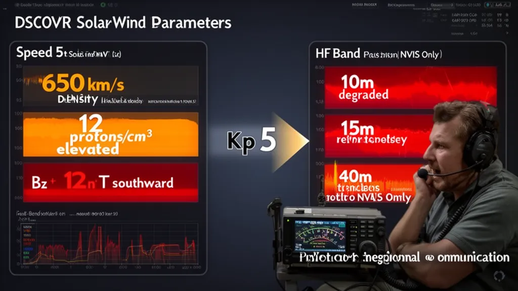
Operator's Verdict: Watch three numbers on the DSCOVR feed: solar wind speed (baseline ~400 km/s — anything above 600 km/s is notable), proton density (spike above 20 p/cm³ signals a shock), and Bz (negative and sustained below −10 nT means trouble is here). DXRadar's solar weather page shows all three in real time with 1-minute cadence. If you see all three go adverse simultaneously, start moving to lower bands.
The Solar Wind and Earth's Magnetosphere
The solar wind is not an occasional event — it is a permanent, continuous outflow of ionized plasma from the Sun's corona that fills the entire inner solar system. At Earth's orbital distance, it arrives at a baseline speed of 350–450 km/s, carrying a density of roughly 5–10 protons per cubic centimeter (p/cm³) and a proton temperature of approximately 10⁵ K. NASA's and NOAA's datasets from ACE and DSCOVR confirm these as long-term averages across multiple solar cycles.
Earth's magnetosphere is the magnetic bubble that deflects this continuous plasma flow. Without the magnetosphere, Earth's surface would be exposed to a flux of energetic particles that would strip the atmosphere over geological timescales. With the magnetosphere, the solar wind is deflected around the Earth at the magnetopause — the boundary between solar wind plasma and Earth's trapped field, typically located at 8–12 Earth radii on the dayside.
The critical parameter governing how much solar wind energy enters the magnetosphere is the interplanetary magnetic field (IMF) carried by the solar wind — specifically its Bz component: the north-south projection of the IMF vector in the geocentric solar magnetospheric (GSM) coordinate system. This is the number that HF operators need to understand.
When Bz is northward (positive), Earth's dipole field and the IMF are aligned in the same direction. The magnetopause is stable; magnetic reconnection is suppressed; solar wind energy stays outside the magnetosphere. HF propagation is unaffected by this interaction.
When Bz is southward (negative), it is anti-parallel to Earth's dipole field at the subsolar magnetopause. Magnetic reconnection occurs: field lines from Earth's magnetosphere connect to the IMF, opening channels for solar wind plasma to flow into the magnetosphere. This injects energy into the ring current, accelerates particles into the auroral oval, and drives geomagnetic activity — directly degrading HF propagation on high-latitude paths.
DSCOVR: The Early Warning Station at L1
The L1 Lagrange point is the gravitational balance point between the Sun and Earth where a satellite can maintain a stable orbit roughly in line between them. It sits approximately 1.5 million km from Earth — about four times the distance to the Moon. DSCOVR (Deep Space Climate Observatory), a joint NOAA-NASA mission, has occupied this position since 2015 following ACE (Advanced Composition Explorer), which began reporting solar wind data in 1998.
At L1, DSCOVR's FARADAY CUP instrument measures solar wind plasma properties: speed, density, and temperature. Its magnetometer measures the three-dimensional IMF vector. Data is transmitted continuously and arrives at NOAA in approximately 15 minutes; processed products appear on the SWPC Real-Time Solar Wind page with 1-minute cadence.
The key physical fact: solar wind plasma traveling at 400 km/s covers the 1.5 million km from L1 to Earth in approximately:
1,500,000 km ÷ 400 km/s = 3,750 seconds ≈ 62.5 minutes
At 700 km/s (CME-enhanced):
1,500,000 km ÷ 700 km/s ≈ 35.7 minutes
At 1,200 km/s (extreme fast CME):
1,500,000 km ÷ 1,200 km/s ≈ 20.8 minutes
This travel time is the storm warning window. When DSCOVR detects a shock — a sudden increase in density and speed combined with compressed IMF — NOAA can issue a geomagnetic storm watch with 20–60 minutes of lead time. That is the window in which an informed HF operator can move to lower bands, adjust antenna configuration, and notify a net about impending degradation.
Pro Tip: Set a browser bookmark to the NOAA SWPC real-time solar wind page or monitor it through DXRadar's solar weather panel. The three-parameter view — speed (km/s), density (p/cm³), and Bz (nT) — gives you everything you need. Check it before any DX session lasting more than one hour, particularly if there has been recent M- or X-class flare activity or a known CME in transit.
Reading the Three Key Solar Wind Parameters
Speed (km/s)
Solar wind speed at L1 ranges from approximately 250 km/s (slow, quiet sun) to over 1,500 km/s (extreme fast CME). DSCOVR measures this directly from the Doppler shift of solar wind protons.
| Speed Range | Significance for HF |
|---|---|
| 250–450 km/s | Background. No direct HF impact expected. |
| 450–600 km/s | Elevated. May indicate leading edge of high-speed stream. Monitor Bz. |
| 600–800 km/s | High. CME or high-speed stream arrival. Kp likely rising to 4–6. |
| 800–1,000 km/s | Very high. Strong CME. G2–G3 conditions probable if Bz southward. |
| 1,000+ km/s | Extreme. Major CME. G4–G5 possible. HF blackout likely on polar paths. |
Speed alone does not determine geomagnetic impact. A fast solar wind with northward Bz produces minimal geomagnetic effect. A moderate-speed wind (500 km/s) with strongly southward Bz (−20 nT) can drive a G3 storm. Speed is a necessary but not sufficient condition.
Density (protons per cm³)
Baseline solar wind density is 5–10 p/cm³. A sudden increase — a density spike above 20–40 p/cm³ coinciding with a speed increase — is the signature of a shock front: the compressed solar wind ahead of a CME or high-speed stream leading edge. This shock creates a sudden commencement (SC), a sharp spike in ground-level magnetometers observable worldwide within minutes of the shock's arrival at Earth's bow shock.
The density spike itself is not the dangerous part for HF. What follows it is: as the CME body arrives behind the shock, the density returns toward normal but the speed remains elevated and, critically, the Bz component may become sustained-southward. The density spike is therefore a predictor, not the impact event.
Monitoring density in the DSCOVR feed, a density jump from 8 to 35 p/cm³ over five minutes, accompanied by a 200 km/s speed increase, is a CME shock arrival. Start watching Bz immediately — it will determine whether you're about to experience a G1 annoyance or a G4 event.
Bz (nT) — The Most Important Parameter
Bz is the vertical component of the IMF in geocentric solar magnetospheric (GSM) coordinates. It is measured in nanotesla (nT). The baseline oscillates between roughly +5 nT and −5 nT in quiet conditions, typically on timescales of minutes to hours driven by solar wind turbulence.
The thresholds that matter for HF operations, based on NOAA SWPC storm level correlations:
| Bz Value | Duration | Expected Geomagnetic Activity | HF Impact |
|---|---|---|---|
| 0 to −5 nT | Any | Kp 1–2; quiet | None |
| −5 to −10 nT | < 1 hour | Kp 3–4; active | Minor — high-latitude paths may show some degradation |
| −10 to −15 nT | 1–3 hours | Kp 5–6; G1–G2 | Polar routes degraded; aurora to ~60° N |
| −15 to −25 nT | 1–3 hours | Kp 6–7; G2–G3 | HF degradation to ~50° N paths; transpacific 15m disrupted |
| −25 to −40 nT | sustained | Kp 7–9; G3–G5 | Widespread HF blackout; aurora to 45° N or lower |
| < −40 nT | sustained | Kp 9; extreme G5 | Near-total HF blackout poleward of 45° N |
The duration of southward Bz is as important as the magnitude. Reconnection-driven energy input to the magnetosphere is a product of Bz magnitude and duration. A brief spike to −30 nT lasting 10 minutes produces less geomagnetic disturbance than a sustained −15 nT episode lasting 6 hours. The ring current builds on a timescale of hours; the Kp index integrates over 3-hour periods.
This is why a CME with a long flux rope — potentially delivering southward Bz for 12–24 hours — is more damaging to HF than a fast CME with a brief southward interval. The May 2024 G5 storm sustained negative Bz for approximately 24 hours at values reaching −40 to −50 nT, producing the most severe geomagnetic conditions since the Halloween storms of October 2003.
The Classic CME Arrival Signature in DSCOVR Data
Experienced space weather observers learn to recognize a CME arrival in the solar wind data. The sequence is typically:
T+0: Shock arrival (S)
- Density spikes suddenly from ~8 to 20–50+ p/cm³
- Speed jumps 100–400 km/s above preceding baseline
- Bz oscillates wildly — direction unpredictable at this stage
- Ground magnetometers globally show sudden commencement (SC) — a sharp positive jump
T+0 to T+2 hours: Sheath region
- Compressed solar wind between shock and CME body
- Bz is highly variable — can be northward or southward unpredictably
- Density remains elevated; speed elevated
- Geomagnetic activity depends entirely on Bz: if sheath Bz goes south, storm can start here
T+2 to T+12+ hours: CME body (magnetic cloud)
- Speed gradually declining from peak
- Density dropping toward normal
- Bz often rotates systematically — can be northward then southward or vice versa
- If the magnetic cloud rotation delivers southward Bz during this phase, the main storm phase begins
Recovery phase:
- Kp returning toward baseline
- Solar wind speed approaching normal
- Bz stabilizing above zero (northward)
The unpredictability of CME arrival Bz is the central challenge of geomagnetic storm forecasting. Even with perfect CME speed and arrival time prediction, the orientation of the CME's internal magnetic field — which determines whether Bz will be northward or southward — cannot be forecast more than 1–2 hours in advance (the L1 travel time). A perfectly placed CME with northward Bz is a non-event for HF. An apparently modest CME that delivers sustained southward Bz for 18 hours can produce a G4 storm.
High-Speed Streams: The Recurring Disturbance
Not all solar wind enhancements are CME-driven. Coronal holes — open magnetic field regions on the Sun — produce persistent high-speed solar wind streams reaching 600–800 km/s. These streams co-rotate with the Sun, repeating every ~27 days (solar rotation period as seen from Earth) as the coronal hole rotates back into the Earth-facing sector.
High-speed streams produce recurrent geomagnetic storms — predictable Kp increases that repeat on the 27-day recurrence interval. They are generally less intense than CME-driven storms (Kp 5–7 rather than 8–9), but more predictable and longer-lasting: a high-speed stream can produce elevated Kp for 2–4 days as Earth traverses the stream edge and body.
The signature in DSCOVR data is a gradual speed increase over 6–24 hours (unlike the sudden shock of a CME), a moderate density decrease (streams are actually lower density than baseline solar wind), and an irregular but sometimes sustained southward Bz within the stream body. Kp typically reaches 4–6 for an isolated coronal hole stream, producing G1–G2 conditions.
For HF operators, a high-speed stream arriving at a known 27-day cadence is an opportunity: if the last arrival was on March 1 and produced Kp 6 for two days, plan accordingly for the ~March 28 recurrence. Conditions will be degraded; schedule regional 40m operations rather than polar-path DX for those 48 hours.
What This Looks Like on the Radio
The progression from DSCOVR data to on-air experience is direct and fairly fast:
T=0: DSCOVR shows density spike (35 p/cm³), speed jump (520 → 680 km/s), Bz chaotic. This is the shock arrival.
T+15 minutes: NOAA SWPC issues a geomagnetic sudden commencement notice. First ground magnetometer deviations appear.
T+2 hours: Bz in the DSCOVR feed settles at −18 nT. Kp begins rising. G2 watch issued by SWPC.
T+3 hours: Kp reaches 6. On 15m SSB, signals from Japan via polar path — which were S9 an hour ago — begin to fade. By T+3.5 hours, the path is S3 with flutter. European operators on 15m lose Asian contacts.
T+4 hours: Kp reaches 7. 15m is completely dead on north-polar paths. 10m was already quiet. 20m shows intermittent flutter and selective fades on paths crossing >55° N. Operators shift to 40m and 20m on equatorial paths to South America and Africa.
T+6 hours: Bz spikes to −28 nT. Kp forecast: 8. G4 watch upgraded from G3. 20m trans-Atlantic paths now degraded. VHF operators in northern Europe start seeing aurora scatter on 2m (50–144 MHz CW/SSB), confirming the auroral oval has expanded equatorward.
T+12 hours: Storm peak. 20m functioning only below ~45° N latitude on low-latitude paths. 40m NVIS still reliable for regional contacts. 80m night propagation unaffected (storm-enhanced D-layer is primarily a daytime and high-latitude effect).
T+30 hours: Kp dropping, Bz recovering northward. 20m trans-Atlantic paths gradually returning. 15m to Europe open by T+36 hours. Full recovery by T+48 hours.
Monitoring DSCOVR data throughout this sequence gives a 30–60 minute lead time at each stage — enough to complete pending QSOs, notify the net, or change to a POTA activation plan that uses 40m instead of 15m.
Reading DXRadar's Solar Wind Panel
The DXRadar solar weather page displays DSCOVR-derived solar wind data in real time from NOAA SWPC feeds. The panel shows:
- Speed (km/s): 1-minute cadence, 24-hour trend. Look for sudden jumps > 100 km/s.
- Density (p/cm³): 1-minute cadence. Look for spikes above 20 p/cm³.
- Bz (nT): 1-minute cadence. The most important single number for storm prediction. Color-coded — green for northward, red for southward below threshold.
The aurora page (/solar-weather/aurora) adds the current Kp and K-index trend, which lags the solar wind by 2–3 hours as the magnetosphere responds to the solar wind forcing. Together, the solar wind panel (leading indicator) and Kp (real-time geomagnetic response) give a complete picture.
For operations planning: if Bz is oscillating around zero and speed is below 450 km/s, conditions are quiet and will remain so for the next 1–2 hours at minimum. If Bz just went from +5 to −15 nT over the last 20 minutes, start moving to lower-frequency bands now — storm onset is in progress.
Frequently Asked Questions
What is DSCOVR and why does it matter for ham radio?
DSCOVR is a NOAA/NASA satellite at the L1 Lagrange point, 1.5 million km sunward from Earth. It continuously measures solar wind speed, density, and the IMF Bz component. Because solar wind takes 30–60 minutes to travel from L1 to Earth, DSCOVR data provides advance storm warning. HF operators watching DSCOVR data can anticipate band degradation 30–60 minutes before it occurs, time enough to complete a DX session or switch to more resilient bands.
What is Bz and why does it matter for HF propagation?
Bz is the north-south component of the interplanetary magnetic field carried by the solar wind. When southward (negative), it connects with Earth's magnetic field via magnetic reconnection, injecting solar wind energy into the magnetosphere and driving geomagnetic storms. Sustained Bz below −10 nT for one or more hours typically produces G1–G2 conditions. Bz below −25 nT sustained for several hours produces G3–G5 storms with widespread HF degradation. Northward Bz has minimal effect on propagation.
How much warning does DSCOVR give before a geomagnetic storm?
At 400 km/s solar wind speed, DSCOVR gives approximately 60 minutes of warning. At CME-enhanced speeds of 700 km/s, this shrinks to about 35 minutes. At extreme fast CME speeds above 1,000 km/s, warning time may be only 15–20 minutes. NOAA issues geomagnetic storm watches based on DSCOVR data as soon as the shock is confirmed, typically within minutes of detection.
What solar wind speed indicates a geomagnetic storm is arriving?
Baseline solar wind is 350–450 km/s. A sudden jump above 500 km/s with an accompanying density spike indicates a CME shock or high-speed stream arrival. Speed above 600 km/s with southward Bz typically drives Kp to 5–6 (G1–G2). Speed above 800 km/s with sustained southward Bz can drive G3–G4 conditions. Speed alone is not sufficient — Bz must go and stay southward for a significant storm to develop.