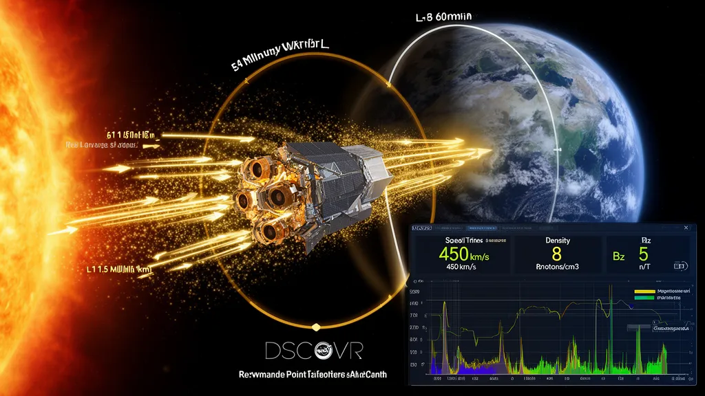
Operator's Verdict: The DSCOVR Bz and solar wind speed data on DXRadar's aurora page show conditions measured 15–60 minutes before they reach Earth. If Bz is currently southward and deepening, a geomagnetic disturbance is imminent. Use the transit time calculation (1,500,000 km ÷ current solar wind speed in km/s) to estimate exactly when storm conditions will arrive.
The L1 Lagrange Point: Why It Is Perfect for Solar Wind Monitoring
The L1 Lagrange point is the first of five gravitational equilibrium points in the Sun-Earth system, identified mathematically by Euler and Lagrange in the 18th century. At L1, the gravitational attractions of the Sun and Earth combine to require an orbital period exactly equal to Earth's, allowing an object to remain roughly stationary relative to Earth while orbiting the Sun.
L1 lies approximately 1,500,000 km from Earth in the direction of the Sun — roughly 1% of the Sun-Earth distance of 150 million km. Objects placed at L1 drift slightly in a halo orbit around the exact Lagrange point (the exact point is unstable against small perturbations; spacecraft use small station-keeping burns to remain in a halo orbit around it).
For solar wind monitoring, L1 is nearly ideal:
- It is permanently sunward of Earth, directly in the path of the solar wind flowing toward Earth
- It is close enough to Earth that data transmission is fast and reliable
- It is far enough from Earth to provide genuine advance warning: at 400 km/s solar wind speed, transit time from L1 to Earth is 1,500,000 ÷ 400 = 3,750 seconds ≈ 62 minutes
- Spacecraft at L1 are outside Earth's magnetosphere and measure unperturbed solar wind
Without L1 monitoring, the first indication of changing solar wind conditions would be when those conditions hit Earth's magnetosphere directly — zero warning time for storms. L1 spacecraft are the only source of definitive lead-time storm warning for the 15–60 minute window between solar wind arrival at L1 and Earth impact.
DSCOVR: NOAA's Primary Solar Wind Sentinel
DSCOVR (Deep Space Climate Observatory) is NOAA's operational space weather monitoring satellite, developed jointly with NASA and the US Air Force. Launched February 11, 2015 aboard a SpaceX Falcon 9 rocket, it reached L1 halo orbit several months later and became NOAA's primary solar wind data source, replacing ACE as the operational standard.
DSCOVR carries two space weather instruments:
PLASMAG (Faraday Cup + Electrostatic Analyzer): Measures solar wind plasma properties — proton speed, density, temperature, and alpha-particle (helium nucleus) fraction. The Faraday cup directly measures particle flux as a function of energy, providing the bulk solar wind speed, proton density (n/cm³), and proton temperature (K) that appear in NOAA's real-time data products.
MAG (Fluxgate Magnetometer): Measures the three-dimensional interplanetary magnetic field vector with precision of approximately 0.1 nT at 1-second cadence. The GSM Bz component computed from MAG data is the most critical operational space weather measurement DSCOVR provides. NOAA transmits MAG data via direct broadcast and ground processing in near-real-time.
DSCOVR data flows from the spacecraft to NOAA ground stations, through processing to NOAA's Space Weather Prediction Center in Boulder, Colorado, and into public real-time data feeds within approximately 1–3 minutes of measurement. DXRadar ingests these NOAA DSCOVR data feeds and displays them on the solar weather aurora page.
DSCOVR also carries an Earth-observing instrument — the EPIC (Earth Polychromatic Imaging Camera) — which provided the iconic "far side" images of Earth frequently used in media. This instrument is not relevant to space weather but explains the "climate observatory" in the mission name.
ACE: The Science Mission That Also Provides Operational Data
ACE (Advanced Composition Explorer) is a NASA science mission launched August 25, 1997, predating DSCOVR by 18 years. It also occupies a halo orbit at L1 and provides continuous solar wind and energetic particle measurements.
ACE's instrument suite is broader than DSCOVR's, originally designed for fundamental heliophysics research:
SWEPAM (Solar Wind Electron Proton Alpha Monitor): Solar wind plasma — speed, density, temperature. Equivalent function to DSCOVR's Faraday cup.
MAG: Magnetic field vector measurement. ACE MAG and DSCOVR MAG produce redundant and cross-validating Bz measurements.
EPAM (Electron, Proton, and Alpha Monitor): Energetic particles in the range ~50 keV to ~5 MeV. Provides early warning of solar proton events and interplanetary shock particle acceleration.
ULEIS/SIS/CRIS: Instrument suite for heavy ion composition and cosmic ray measurements — primarily science instruments of limited operational relevance for real-time HF prediction.
SWICS (Solar Wind Ion Composition Spectrometer): Ion composition ratios that can distinguish CME magnetic cloud plasma from ambient solar wind — a scientific indicator but occasionally used to confirm CME passage.
Before DSCOVR, ACE was NOAA's sole primary real-time solar wind data source. It served this role for 18 years, far exceeding its 2-year design lifetime. ACE continues to operate in 2026 and provides valuable redundancy: when one L1 spacecraft experiences technical issues, the other maintains continuity of the critical solar wind data stream.
NOAA and USAF are planning the SWFO-L1 (Space Weather Follow-On L1) mission to succeed DSCOVR operationally when necessary. The principle — a continuously operated L1 solar wind monitor as a national and international public utility — is firmly established.
What DSCOVR Measures and What It Means for HF Operators
The four DSCOVR parameters most directly relevant to HF propagation are:
Bz (nT) — The Storm Trigger
Bz is the north-south component of the IMF in GSM coordinates. This is the single most operationally important solar wind parameter for HF propagation prediction. When Bz turns negative and sustains below −5 nT, magnetospheric coupling begins. Below −10 nT sustained for 1+ hours, G2 storm conditions develop. Below −20 nT for 30+ minutes, G4 territory.
DSCOVR MAG provides Bz at 1-second cadence in raw telemetry and at 1-minute averages in the standard public product. The 1-minute average is adequate for operational storm monitoring.
What to do with this number: monitor the trend, not just the instantaneous value. Use DXRadar's aurora page Bz trend display. A Bz that has been at −8 nT for 45 minutes is more significant than an instantaneous −8 nT reading following an hour at +5 nT.
Solar Wind Speed (km/s) — Context and Lead Time
Solar wind speed measured by DSCOVR's PLASMAG defines:
- How energetic the current solar wind interaction is — high-speed streams carry more kinetic energy and are more geoeffective for a given Bz value
- The current L1-to-Earth transit time — critical for timing storm onset predictions
- Whether a speed enhancement indicates CME or CIR arrival — a speed jump from ambient 400 to 600+ km/s signals a significant new solar wind structure arriving
| Speed (km/s) | Interpretation | Typical L1→Earth Transit |
|---|---|---|
| 280–350 | Very slow; quiet | 71–89 min |
| 350–450 | Normal slow solar wind | 55–71 min |
| 450–550 | Moderate; elevated | 45–55 min |
| 550–650 | Fast stream / CIR arrival likely | 38–45 min |
| 650–800 | Fast stream peak or early CME | 31–38 min |
| 800–1,200 | CME shock or extreme fast stream | 21–31 min |
| >1,200 | Major CME shock | <21 min |
Proton Density (p/cm³) — Shock and CME Indicators
Proton density under quiet conditions is typically 3–10 p/cm³. Departures from this range indicate specific solar wind structures:
Density spike (>20 p/cm³): Compressed plasma at a CIR boundary or CME sheath. Density spikes often accompany the initial shock arrival of a CME, coinciding with a speed jump and often a chaotic Bz. A density spike followed by smooth declining density and a coherent rotating magnetic field = CME magnetic cloud passage.
Density drop (<3 p/cm³): Inside a CME magnetic cloud (the rarefied interior of the flux rope). Low density combined with elevated field magnitude and smooth Bz rotation are diagnostic of magnetic cloud passage.
Background density elevation: Sustained density above 10 p/cm³ often accompanies solar maximum conditions when the corona is more disturbed and solar wind is generally more complex.
Proton density alone has modest direct effect on HF propagation. Its value is primarily as a CME/CIR diagnostic — in combination with speed and Bz, it helps identify what solar wind structure is arriving and predict what will follow.
Proton Temperature (K) — CME Identification
Solar wind proton temperature follows a predictable relationship with speed in ambient solar wind: faster streams are hotter. A simple temperature-speed relationship T_expected = (0.031 × V - 4.39) × 10⁴ K (approximately, per ACE mission solar wind characterization) defines the expected temperature for a given speed.
CME magnetic cloud plasma is typically anomalously cold relative to this expectation — the expanding flux rope cools the plasma during transit. When DSCOVR measures proton temperatures significantly below the expected value for the observed speed, CME magnetic cloud passage is the most likely explanation.
For operational HF planning, proton temperature helps answer: "Is this elevated solar wind speed due to a CIR (expected temperature, will produce moderate sustained disturbance) or a CME (anomalously cold, structured Bz, more intense but possibly shorter duration)?" The answer shapes the forecast.
The Warning Time Calculation in Practice
The transit time from L1 to Earth's magnetopause is:
Transit time (seconds) = 1,500,000 km ÷ solar wind speed (km/s)
Converting to minutes: divide the result by 60.
Worked examples:
- 400 km/s (quiet slow solar wind): 1,500,000 ÷ 400 = 3,750 sec = 62.5 minutes
- 500 km/s (moderate fast stream): 1,500,000 ÷ 500 = 3,000 sec = 50 minutes
- 650 km/s (fast coronal hole stream): 1,500,000 ÷ 650 = 2,308 sec = 38 minutes
- 900 km/s (fast CME shock): 1,500,000 ÷ 900 = 1,667 sec = 28 minutes
- 1,500 km/s (extreme CME): 1,500,000 ÷ 1,500 = 1,000 sec = 17 minutes
This warning time is the gap between what DSCOVR measures and when those conditions begin producing geomagnetic effects at Earth. "Begin producing" is the operative phrase: the magnetosphere responds within minutes of solar wind impact, but storm-level Kp takes 30–90 minutes to build from initial solar wind coupling. The total lead time from first DSCOVR detection to full storm development is thus typically 45–150 minutes from initial Bz southward turn, depending on solar wind speed and storm intensity.
During a NOAA geomagnetic storm watch (CME inbound), open DXRadar's aurora page and calculate the current transit time: 1,500,000 ÷ current solar wind speed (km/s). Check back at that interval after a Bz southward turn — if Bz is still south, storm onset is now imminent. The math takes 10 seconds and gives you the most accurate near-term storm timing available.
Data Flow: From Spacecraft to Your Browser
Understanding the data pipeline helps set realistic expectations for latency and data gaps:
- DSCOVR instruments sample at 1-second to 1-minute cadence depending on the parameter
- Telemetry transmitted to NOAA ground stations via X-band downlink
- NOAA Space Weather Prediction Center processes incoming data and publishes real-time data products (typically 1–3 minute latency from measurement to public availability)
- DXRadar backend fetches NOAA SWPC real-time data feeds on a regular polling schedule
- DXRadar frontend displays the data on aurora and solar weather pages
Occasional data gaps occur — typically a few minutes to tens of minutes — due to telemetry dropouts, ground station handoffs, or instrument mode changes. During these gaps, NOAA flags the data as unavailable rather than interpolating. DXRadar handles these gaps gracefully, showing the most recent valid measurement with appropriate timestamp.
When DSCOVR has a significant anomaly, ACE data can serve as backup. NOAA maintains contingency procedures to switch primary data sourcing to ACE when needed. The two spacecraft have slightly different orbital positions in their L1 halo orbits and may observe somewhat different solar wind micro-structure, but for operational storm monitoring they are interchangeable.
Interpreting CME Arrival at L1: A Signature Sequence
CME shock arrival at L1 produces a characteristic sequence in DSCOVR data, detectable within minutes of passage:
Phase 1 — Shock front (minutes):
- Solar wind speed jumps suddenly (50–500 km/s increase)
- Proton density spikes (often 2–10× ambient)
- IMF magnitude increases sharply
- Bz becomes erratic — rapid oscillations between northward and southward as the compressed sheath region passes
Phase 2 — CME sheath (hours):
- Elevated speed and density persist
- Bz continues fluctuating but often has a southward bias
- This phase can drive geomagnetic activity if the sheath Bz dips significantly southward
Phase 3 — Magnetic cloud (12–24 hours):
- Proton density drops to below-ambient levels
- Proton temperature drops below the speed-temperature relationship prediction
- IMF magnitude remains elevated
- Bz rotates smoothly through a large angular range — this is the CME flux rope passing over Earth
- If the rotation includes a sustained southward Bz phase, this is when the most intense storm activity occurs
Phase 4 — Trailing region:
- Solar wind parameters relax toward ambient
- Bz returns to low-amplitude fluctuation
- Storm recovery begins at Earth as Bz recovers northward
Recognizing Phase 1 in real-time DSCOVR data is the most actionable skill for an HF operator during a CME event. The speed jump and density spike are unmistakable. At that point, storm onset at Earth is 15–60 minutes away, and the character of the subsequent storm is already being determined by the Bz behavior unfolding in the DSCOVR data stream.
Frequently Asked Questions
What is the L1 Lagrange point?
L1 is the first Lagrange point, a gravitational equilibrium location between the Sun and Earth approximately 1.5 million km sunward of Earth (~1% of the Sun-Earth distance). An object at L1 orbits the Sun at the same angular rate as Earth but remains roughly stationary relative to Earth, making it an ideal location for continuous upstream solar wind monitoring.
How much warning does DSCOVR provide before solar wind reaches Earth?
DSCOVR at L1 provides approximately 15–60 minutes of advance warning before measured solar wind conditions reach Earth. At typical solar wind speed of 400 km/s, the transit from L1 to Earth takes about 62 minutes. At 800 km/s (fast stream or CME arrival), lead time drops to approximately 31 minutes.
What is the difference between DSCOVR and ACE?
Both DSCOVR and ACE are positioned at L1. DSCOVR (launched 2015) is NOAA's primary operational solar wind monitor, providing real-time Bz, solar wind speed, and proton density. ACE (launched 1997) is a NASA science mission with broader instrument coverage including energetic particle composition and energetic solar proton flux. ACE data supplements DSCOVR and provides redundancy.
What DSCOVR data does DXRadar display?
DXRadar's aurora and solar weather pages display real-time Bz, solar wind speed, and proton density sourced from NOAA's DSCOVR data stream. These update at the same cadence as NOAA's published product — typically 1-minute resolution. The Bz gauge, wind speed indicator, and Kp index together provide the key indicators for near-term HF propagation quality.
How do I calculate solar wind transit time from L1 to Earth?
Divide the L1-Earth distance (approximately 1,500,000 km) by the current solar wind speed in km/s. At 400 km/s: 1,500,000 ÷ 400 = 3,750 seconds ≈ 62 minutes. At 700 km/s: 1,500,000 ÷ 700 ≈ 36 minutes. At 1,500 km/s (fast CME): 1,500,000 ÷ 1,500 = 17 minutes. Transit time is the lead time between what DSCOVR measures and when those conditions arrive at Earth.
What does a solar wind speed spike on DSCOVR indicate?
A sudden jump in solar wind speed — from ambient 400 km/s to 600+ km/s — typically indicates either a corotating interaction region (CIR) boundary or a CME shock arrival at L1. Combined with a simultaneous Bz southward turn and proton density increase, it is a reliable signature of CME shock passage. Storm conditions at Earth will follow within 15–60 minutes.